11. Point-Stat Tool
11.1. Introduction
The Point-Stat tool provides verification statistics for forecasts at observation points (as opposed to over gridded analyses). The Point-Stat tool matches gridded forecasts to point observation locations and supports several different interpolation options. The tool then computes continuous, categorical, spatial, and probabilistic verification statistics. The categorical and probabilistic statistics generally are derived by applying a threshold to the forecast and observation values. Confidence intervals - representing the uncertainty in the verification measures - are computed for the verification statistics.
Scientific and statistical aspects of the Point-Stat tool are discussed in the following section. Practical aspects of the Point-Stat tool are described in Section 11.3.
11.2. Scientific and Statistical Aspects
The statistical methods and measures computed by the Point-Stat tool are described briefly in this section. In addition, Section 11.2.1 discusses the various interpolation options available for matching the forecast grid point values to the observation points. The statistical measures computed by the Point-Stat tool are described briefly in Section 11.2.4 and in more detail in Appendix C, Section 34. Section 11.2.5 describes the methods for computing confidence intervals that are applied to some of the measures computed by the Point-Stat tool; more detail on confidence intervals is provided in Appendix D, Section 35.
11.2.1. Interpolation/Matching Methods
This section provides information about the various methods available in MET to match gridded model output to point observations. Matching in the vertical and horizontal are completed separately using different methods.
In the vertical, if forecasts and observations are at the same vertical level, then they are paired as-is. If any discrepancy exists between the vertical levels, then the forecasts are interpolated to the level of the observation. The vertical interpolation is done in the natural log of pressure coordinates, except for specific humidity, which is interpolated using the natural log of specific humidity in the natural log of pressure coordinates. Vertical interpolation for heights above ground are done linear in height coordinates. When forecasts are for the surface, no interpolation is done. They are matched to observations with message types that are mapped to SURFACE in the message_type_group_map configuration option. By default, the surface message types include ADPSFC, SFCSHP, and MSONET. The regular expression is applied to the message type list at the message_type_group_map. The derived message types from the time summary (“ADPSFC_MIN_hhmmss” and “ADPSFC_MAX_hhmmss”) are accepted as “ADPSFC”.
To match forecasts and observations in the horizontal plane, the user can select from a number of methods described below. Many of these methods require the user to define the width of the forecast grid W, around each observation point P, that should be considered. In addition, the user can select the interpolation shape, either a SQUARE or a CIRCLE. For example, a square of width 2 defines the 2 x 2 set of grid points enclosing P, or simply the 4 grid points closest to P. A square of width of 3 defines a 3 x 3 square consisting of 9 grid points centered on the grid point closest to P. Figure 11.1 provides illustration. The point P denotes the observation location where the interpolated value is calculated. The interpolation width W, shown is five.
This section describes the options for interpolation in the horizontal.
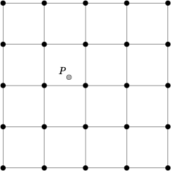
Figure 11.1 Diagram illustrating matching and interpolation methods used in MET. See text for explanation.
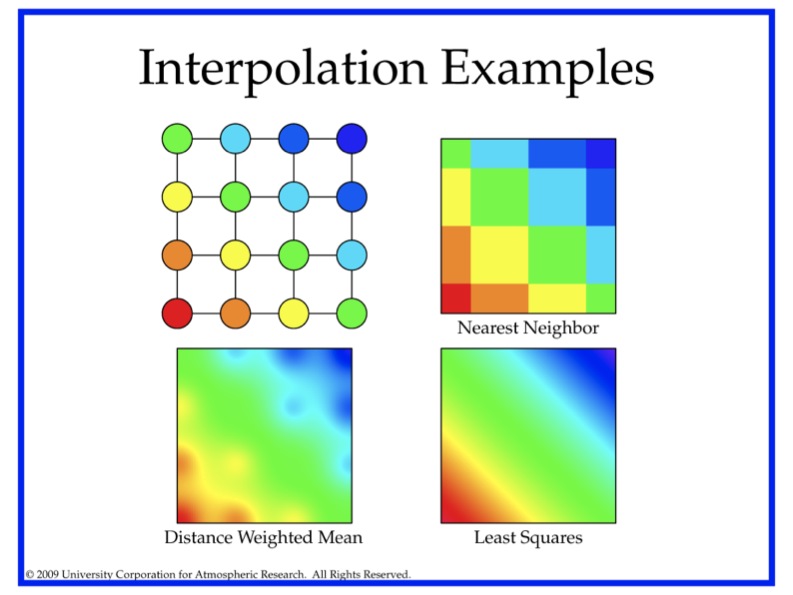
Figure 11.2 Illustration of some matching and interpolation methods used in MET. See text for explanation.
Nearest Neighbor
The forecast value at P is assigned the value at the nearest grid point. No interpolation is performed. Here, “nearest” means spatially closest in horizontal grid coordinates. This method is used by default when the interpolation width, W, is set to 1.
Geography Match
The forecast value at P is assigned the value at the nearest grid point in the interpolation area where the land/sea mask and topography criteria are satisfied.
Gaussian
The forecast value at P is a weighted sum of the values in the interpolation area. The weight given to each forecast point follows the Gaussian distribution with nearby points contributing more the far away points. The shape of the distribution is configured using sigma.
When used for regridding, with the regrid configuration option, or smoothing, with the interp configuration option in grid-to-grid comparisons, the Gaussian method is named MAXGAUSS and is implemented as a 2-step process. First, the data is regridded or smoothed using the maximum value interpolation method described below, where the width and shape define the interpolation area. Second, the Gaussian smoother, defined by the gaussian_dx and gaussian_radius configuration options, is applied.
Minimum value
The forecast value at P is the minimum of the values in the interpolation area.
Maximum value
The forecast value at P is the maximum of the values in the interpolation area.
Distance-weighted mean
The forecast value at P is a weighted sum of the values in the interpolation area. The weight given to each forecast point is the reciprocal of the square of the distance (in grid coordinates) from P. The weighted sum of forecast values is normalized by dividing by the sum of the weights.
Unweighted mean
This method is similar to the distance-weighted mean, except all the weights are equal to 1. The distance of any point from P is not considered.
Median
The forecast value at P is the median of the forecast values in the interpolation area.
Least-Squares Fit
To perform least squares interpolation of a gridded field at a location P, MET uses an WxW subgrid centered (as closely as possible) at P. Figure 11.1 shows the case where W = 5.
If we denote the horizontal coordinate in this subgrid by x, and vertical coordinate by y, then we can assign coordinates to the point P relative to this subgrid. These coordinates are chosen so that the center of the grid is. For example, in Figure 11.1, P has coordinates (-0.4, 0.2). Since the grid is centered near P, the coordinates of P should always be at most 0.5 in absolute value. At each of the vertices of the grid (indicated by black dots in the figure), we have data values. We would like to use these values to interpolate a value at P. We do this using least squares. If we denote the interpolated value by z, then we fit an expression of the form \(z=\alpha (x) + \beta (y) + \gamma\) over the subgrid. The values of \(\alpha, \beta, \gamma\) are calculated from the data values at the vertices. Finally, the coordinates (x,y) of P are substituted into this expression to give z, our least squares interpolated data value at P.
Bilinear Interpolation
This method is performed using the four closest grid squares. The forecast values are interpolated linearly first in one dimension and then the other to the location of the observation.
Upper Left, Upper Right, Lower Left, Lower Right Interpolation
This method is performed using the four closest grid squares. The forecast values are interpolated to the specified grid point.
Best Interpolation
The forecast value at P is chosen as the grid point inside the interpolation area whose value most closely matches the observation value.
11.2.2. HiRA Framework
The Point-Stat tool has been enhanced to include the High Resolution Assessment (HiRA) verification logic (Mittermaier, 2014). HiRA is analogous to neighborhood verification but for point observations. The HiRA logic interprets the forecast values surrounding each point observation as an ensemble forecast. These ensemble values are processed in three ways. First, the ensemble continuous statistics (ECNT), the observation rank statistics (ORANK) and the ranked probability score (RPS) line types are computed directly from the ensemble values. Second, for each categorical threshold specified, a fractional coverage value is computed as the ratio of the nearby forecast values that meet the threshold criteria. Point-Stat evaluates those fractional coverage values as if they were a probability forecast. When applying HiRA, users should enable the matched pair (MPR), probabilistic (PCT, PSTD, PJC, or PRC), continuous ensemble statistics (ECNT), observation rank statistics (ORANK) or ranked probability score (RPS) line types in the output_flag dictionary. The number of probabilistic HiRA output lines is determined by the number of categorical forecast thresholds and HiRA neighborhood widths chosen.
The HiRA framework provides a unique method for evaluating models in the neighborhood of point observations, allowing for some spatial and temporal uncertainty in the forecast and/or the observations. Additionally, the HiRA framework can be used to compare deterministic forecasts to ensemble forecasts. In MET, the neighborhood is a circle or square centered on the grid point closest to the observation location. An event is defined, then the proportion of points with events in the neighborhood is calculated. This proportion is treated as an ensemble probability, though it is likely to be uncalibrated.
Figure 11.3 shows a couple of examples of how the HiRA proportion is derived at a single model level using square neighborhoods. Events (in our case, model accretion values > 0) are separated from non-events (model accretion value = 0). Then, in each neighborhood, the total proportion of events is calculated. In the leftmost panel, four events exist in the 25 point neighborhood, making the HiRA proportion is 4/25 = 0.16. For the neighborhood of size 9 centered in that same panel, the HiRA proportion is 1/9. In the right panel, the size 25 neighborhood has HiRA proportion of 6/25, with the centered 9-point neighborhood having a HiRA value of 2/9. To extend this method into 3-dimensions, all layers within the user-defined layer are also included in the calculation of the proportion in the same manner.

Figure 11.3 Example showing how HiRA proportions are calculated.
Often, the neighborhood size is chosen so that multiple models to be compared have approximately the same horizontal resolution. Then, standard metrics for probabilistic forecasts, such as Brier Score, can be used to compare those forecasts. HiRA was developed using surface observation stations so the neighborhood lies completely within the horizontal plane. With any type of upper air observation, the vertical neighborhood must also be defined.
11.2.3. SEEPS Scores
The Stable Equitable Error in Probability Space (SEEPS) was devised for monitoring global deterministic forecasts of precipitation against the WMO gauge network (Rodwell et al., 2010; Haiden et al., 2012) and is a multi-category score which uses a climatology to account for local variations in behavior. Since the score uses probability space to define categories using the climatology, it can be aggregated over heterogeneous climate regions. Even though it was developed for use with precipitation forecasts, in principle it could be applied to any forecast parameter for which a sufficiently long time period of observations exists to create a suitable climatology. The computation of SEEPS for precipitation is only supported for now.
For use with precipitation, three categories are used, named ‘dry’, ‘light’ and ‘heavy’. The ‘dry’ category is defined (using the WMO observing guidelines) with any accumulation (rounded to the nearest 0.1 millimeter) that is less than or equal to 0.2 mm. The remaining precipitation is divided into ‘light’ and ‘heavy’ categories whose thresholds are with respect to a climatology and thus location specific. The light precipitation is defined to occur twice as often as heavy precipitation.
When calculating a single SEEPS value over observing stations for a particular region, the scores should have a density weighting applied which accounts for uneven station distribution in the region of interest (see Section 9.1 in Rodwell et al., 2010). This density weighting has not yet been implemented in MET. Global precipitation climatologies calculated from the WMO SYNOP records from 1980-2009 are supplied with the release. At the moment, a 24-hour climatology is available (valid at 00 UTC or 12 UTC), but in future a 6-hour climatology will become available.
11.2.4. Statistical Measures
The Point-Stat tool computes a wide variety of verification statistics. Broadly speaking, these statistics can be subdivided into statistics for categorical variables and statistics for continuous variables. The categories of measures are briefly described here; specific descriptions of the measures are provided in Appendix C, Section 34. Additional information can be found in Wilks (2011) and Jolliffe and Stephenson (2012), and at Collaboration for Australian Weather and Climate Research. Forecast Verification - Issues, Methods and FAQ web page.
In addition to these verification measures, the Point-Stat tool also computes partial sums and other FHO statistics that are produced by the NCEP verification system. These statistics are also described in Appendix C, Section 34.
11.2.4.1. Measures for Categorical Variables
Categorical verification statistics are used to evaluate forecasts that are in the form of a discrete set of categories rather than on a continuous scale. If the original forecast is continuous, the user may specify one or more thresholds in the configuration file to divide the continuous measure into categories. Currently, Point-Stat computes categorical statistics for variables in two or more categories. The special case of dichotomous (i.e., 2-category) variables has several types of statistics calculated from the resulting contingency table and are available in the CTS output line type. For multi-category variables, fewer statistics can be calculated so these are available separately, in line type MCTS. Categorical variables can be intrinsic (e.g., rain/no-rain) or they may be formed by applying one or more thresholds to a continuous variable (e.g., temperature < 273.15 K or cloud coverage percentages in 10% bins). See Appendix C, Section 34 for more information.
11.2.4.2. Measures for Continuous Variables
For continuous variables, many verification measures are based on the forecast error (i.e., f - o). However, it also is of interest to investigate characteristics of the forecasts, and the observations, as well as their relationship. These concepts are consistent with the general framework for verification outlined by Murphy and Winkler (1987). The statistics produced by MET for continuous forecasts represent this philosophy of verification, which focuses on a variety of aspects of performance rather than a single measure. See Appendix C, Section 34 for specific information.
A user may wish to eliminate certain values of the forecasts from the calculation of statistics, a process referred to here as``’conditional verification’’. For example, a user may eliminate all temperatures above freezing and then calculate the error statistics only for those forecasts of below freezing temperatures. Another common example involves verification of wind forecasts. Since wind direction is indeterminate at very low wind speeds, the user may wish to set a minimum wind speed threshold prior to calculating error statistics for wind direction. The user may specify these thresholds in the configuration file to specify the conditional verification. Thresholds can be specified using the usual Fortran conventions (<, <=, ==, !-, >=, or >) followed by a numeric value. The threshold type may also be specified using two letter abbreviations (lt, le, eq, ne, ge, gt). Further, more complex thresholds can be achieved by defining multiple thresholds and using && or || to string together event definition logic. The forecast and observation threshold can be used together according to user preference by specifying one of: UNION, INTERSECTION, or SYMDIFF (symmetric difference).
11.2.4.3. Measures for Probabilistic Forecasts and Dichotomous Outcomes
For probabilistic forecasts, many verification measures are based on reliability, accuracy and bias. However, it also is of interest to investigate joint and conditional distributions of the forecasts and the observations, as in Wilks (2011). See Appendix C, Section 34 for specific information.
Probabilistic forecast values are assumed to have a range of either 0 to 1 or 0 to 100. If the max data value is > 1, we assume the data range is 0 to 100, and divide all the values by 100. If the max data value is <= 1, then we use the values as is. Further, thresholds are applied to the probabilities with equality on the lower end. For example, with a forecast probability p, and thresholds t1 and t2, the range is defined as: t1 <= p < t2. The exception is for the highest set of thresholds, when the range includes 1: t1 <= p <= 1. To make configuration easier, in METv6.0, these probabilities may be specified in the configuration file as a list (>=0.00,>=0.25,>=0.50,>=0.75,>=1.00) or using shorthand notation (==0.25) for bins of equal width.
When the “prob” entry is set as a dictionary to define the field of interest, setting “prob_as_scalar = TRUE” indicates that this data should be processed as regular scalars rather than probabilities. For example, this option can be used to compute traditional 2x2 contingency tables and neighborhood verification statistics for probability data. It can also be used to compare two probability fields directly.
11.2.4.4. Measures for Comparison Against Climatology
For each of the types of statistics mentioned above (categorical, continuous, and probabilistic), it is possible to calculate measures of skill relative to climatology. MET will accept a climatology file provided by the user, and will evaluate it as a reference forecast. Further, anomalies, i.e. departures from average conditions, can be calculated. As with all other statistics, the available measures will depend on the nature of the forecast. Common statistics that use a climatological reference include: the mean squared error skill score (MSESS), the Anomaly Correlation (ANOM_CORR and ANOM_CORR_UNCNTR), scalar and vector anomalies (SAL1L2 and VAL1L2), continuous ranked probability skill score (CRPSS and CRPSS_EMP), Brier Skill Score (BSS) (Wilks, 2011; Mason, 2004).
Often, the sample climatology is used as a reference by a skill score. The sample climatology is the average over all included observations and may be transparent to the user. This is the case in most categorical skill scores. The sample climatology will probably prove more difficult to improve upon than a long term climatology, since it will be from the same locations and time periods as the forecasts. This may mask legitimate forecast skill. However, a more general climatology, perhaps covering many years, is often easier to improve upon and is less likely to mask real forecast skill.
11.2.5. Statistical Confidence Intervals
A single summary score gives an indication of the forecast performance, but it is a single realization from a random process that neglects uncertainty in the score’s estimate. That is, it is possible to obtain a good score, but it may be that the “good” score was achieved by chance and does not reflect the “true” score. Therefore, when interpreting results from a verification analysis, it is imperative to analyze the uncertainty in the realized scores. One good way to do this is to utilize confidence intervals. A confidence interval indicates that if the process were repeated many times, say 100, then the true score would fall within the interval \(100(1-\alpha)\%\) of the time. Typical values of \(\alpha\) are 0.01, 0.05, and 0.10. The Point-Stat tool allows the user to select one or more specific \(\alpha\)-values to use.
For continuous fields (e.g., temperature), it is possible to estimate confidence intervals for some measures of forecast performance based on the assumption that the data, or their errors, are normally distributed. The Point-Stat tool computes confidence intervals for the following summary measures: forecast mean and standard deviation, observation mean and standard deviation, correlation, mean error, and the standard deviation of the error. In the case of the respective means, the central limit theorem suggests that the means are normally distributed, and this assumption leads to the usual \(100(1-\alpha)\%\) confidence intervals for the mean. For the standard deviations of each field, one must be careful to check that the field of interest is normally distributed, as this assumption is necessary for the interpretation of the resulting confidence intervals.
For the measures relating the two fields (i.e., mean error, correlation and standard deviation of the errors), confidence intervals are based on either the joint distributions of the two fields (e.g., with correlation) or on a function of the two fields. For the correlation, the underlying assumption is that the two fields follow a bivariate normal distribution. In the case of the mean error and the standard deviation of the mean error, the assumption is that the errors are normally distributed, which for continuous variables, is usually a reasonable assumption, even for the standard deviation of the errors.
Bootstrap confidence intervals for any verification statistic are available in MET. Bootstrapping is a nonparametric statistical method for estimating parameters and uncertainty information. The idea is to obtain a sample of the verification statistic(s) of interest (e.g., bias, ETS, etc.) so that inferences can be made from this sample. The assumption is that the original sample of matched forecast-observation pairs is representative of the population. Several replicated samples are taken with replacement from this set of forecast-observation pairs of variables (e.g., precipitation, temperature, etc.), and the statistic(s) are calculated for each replicate. That is, given a set of n forecast-observation pairs, we draw values at random from these pairs, allowing the same pair to be drawn more than once, and the statistic(s) is (are) calculated for each replicated sample. This yields a sample of the statistic(s) based solely on the data without making any assumptions about the underlying distribution of the sample. It should be noted, however, that if the observed sample of matched pairs is dependent, then this dependence should be taken into account somehow. Currently, the confidence interval methods in MET do not take into account dependence, but future releases will support a robust method allowing for dependence in the original sample. More detailed information about the bootstrap algorithm is found in the Appendix D, Section 35. Note that MET writes temporary files whenever bootstrap confidence intervals are computed, as described in Contributor's Guide Section 3.1.3.
Confidence intervals can be calculated from the sample of verification statistics obtained through the bootstrap algorithm. The most intuitive method is to simply take the appropriate quantiles of the sample of statistic(s). For example, if one wants a 95% CI, then one would take the 2.5 and 97.5 percentiles of the resulting sample. This method is called the percentile method, and has some nice properties. However, if the original sample is biased and/or has non-constant variance, then it is well known that this interval is too optimistic. The most robust, accurate, and well-behaved way to obtain accurate CIs from bootstrapping is to use the bias corrected and adjusted percentile method (or BCa). If there is no bias, and the variance is constant, then this method will yield the usual percentile interval. The only drawback to the approach is that it is computationally intensive. Therefore, both the percentile and BCa methods are available in MET, with the considerably more efficient percentile method being the default.
The only other option associated with bootstrapping currently available in MET is to obtain replicated samples smaller than the original sample (i.e., to sample m<n points at each replicate). Ordinarily, one should use m=n, and this is the default. However, there are cases where it is more appropriate to use a smaller value of m (e.g., when making inference about high percentiles of the original sample). See Gilleland (2010) for more information and references about this topic.
MET provides parametric confidence intervals based on assumptions of normality for the following categorical statistics:
Base Rate
Forecast Mean
Accuracy
Probability of Detection
Probability of Detection of the non-event
Probability of False Detection
False Alarm Ratio
Critical Success Index
Hanssen-Kuipers Discriminant
Odds Ratio
Log Odds Ratio
Odds Ratio Skill Score
Extreme Dependency Score
Symmetric Extreme Dependency Score
Extreme Dependency Index
Symmetric Extremal Dependency Index
MET provides parametric confidence intervals based on assumptions of normality for the following continuous statistics:
Forecast and Observation Means
Forecast, Observation, and Error Standard Deviations
Pearson Correlation Coefficient
Mean Error
MET provides parametric confidence intervals based on assumptions of normality for the following probabilistic statistics:
Brier Score
Base Rate
MET provides non-parametric bootstrap confidence intervals for many categorical and continuous statistics. Kendall’s Tau and Spearman’s Rank correlation coefficients are the only exceptions. Computing bootstrap confidence intervals for these statistics would be computationally unrealistic.
For more information on confidence intervals pertaining to verification measures, see Wilks (2011), Jolliffe and Stephenson (2012), and Bradley (2008).
11.3. Practical Information
The Point-Stat tool is used to perform verification of a gridded model field using point observations. The gridded model field to be verified must be in one of the supported file formats. The point observations must be formatted as the NetCDF output of the point reformatting tools described in Section 7. The Point-Stat tool provides the capability of interpolating the gridded forecast data to the observation points using a variety of methods as described in Section 11.2.1. The Point-Stat tool computes a number of continuous statistics on the matched pair data as well as discrete statistics once the matched pair data have been thresholded.
If no matched pairs are found for a particular verification task, a report listing counts for reasons why the observations were not used is written to the log output at the default verbosity level of 2. If matched pairs are found, this report is written at verbosity level 3. Inspecting these rejection reason counts is the first step in determining why Point-Stat found no matched pairs. The order of the log messages matches the order in which the processing logic is applied. Start from the last log message and work your way up, considering each of the non-zero rejection reason counts.
11.3.1. point_stat Usage
The usage statement for the Point-Stat tool is shown below:
Usage: point_stat
       fcst_file
       obs_file
       config_file
       [-point_obs file]
       [-obs_valid_beg time]
       [-obs_valid_end time]
       [-outdir path]
       [-log file]
       [-v level]
point_stat has three required arguments and can take many optional ones.
11.3.1.1. Required Arguments for point_stat
The fcst_file argument names the gridded file in either GRIB or NetCDF containing the model data to be verified.
The obs_file argument indicates the MET NetCDF point observation file to be used for verifying the model. Python embedding for point observations is also supported, as described in Section 37.4.2.
The config_file argument indicates the name of the configuration file to be used. The contents of the configuration file are discussed below.
11.3.1.2. Optional Arguments for point_stat
The -point_obs file may be used to pass additional NetCDF point observation files to be used in the verification. Python embedding for point observations is also supported, as described in Section 37.4.2.
The -obs_valid_beg time option in YYYYMMDD[_HH[MMSS]] format sets the beginning of the observation matching time window, overriding the configuration file setting.
The -obs_valid_end time option in YYYYMMDD[_HH[MMSS]] format sets the end of the observation matching time window, overriding the configuration file setting.
The -outdir path indicates the directory where output files should be written.
The -log file option directs output and errors to the specified log file. All messages will be written to that file as well as standard out and error. Thus, users can save the messages without having to redirect the output on the command line. The default behavior is no log file.
The -v level option indicates the desired level of verbosity. The value of “level” will override the default setting of 2. Setting the verbosity to 0 will make the tool run with no log messages, while increasing the verbosity will increase the amount of logging.
An example of the point_stat calling sequence is shown below:
point_stat sample_fcst.grb \
sample_pb.nc \
PointStatConfig
In this example, the Point-Stat tool evaluates the model data in the sample_fcst.grb GRIB file using the observations in the NetCDF output of PB2NC, sample_pb.nc, applying the configuration options specified in the PointStatConfig file.
11.3.2. point_stat Configuration File
The default configuration file for the Point-Stat tool named PointStatConfig_default can be found in the installed share/met/config directory. Another version is located in scripts/config. We encourage users to make a copy of these files prior to modifying their contents. The contents of the configuration file are described in the subsections below.
Note that environment variables may be used when editing configuration files, as described in the Section 5.1.1.
model          = "FCST";
desc           = "NA";
regrid         = { ... }
climo_mean     = { ... }
climo_stdev    = { ... }
climo_cdf      = { ... }
obs_window     = { beg = -5400; end =  5400; }
mask           = { grid = [ "FULL" ]; poly = []; sid = []; }
ci_alpha       = [ 0.05 ];
boot           = { interval = PCTILE; rep_prop = 1.0; n_rep = 1000;
                   rng = "mt19937"; seed = ""; }
interp         = { vld_thresh = 1.0; shape = SQUARE;
                   type = [ { method = NEAREST; width = 1; } ]; }
censor_thresh  = [];
censor_val     = [];
mpr_column     = [];
mpr_thresh     = [];
eclv_points    = 0.05;
hss_ec_value   = NA;
rank_corr_flag = TRUE;
sid_inc        = [];
sid_exc        = [];
duplicate_flag = NONE;
obs_quality_inc  = [];
obs_quality_exc  = [];
obs_summary    = NONE;
obs_perc_value = 50;
message_type_group_map = [...];
tmp_dir        = "/tmp";
output_prefix  = "";
version        = "VN.N";
The configuration options listed above are common to multiple MET tools and are described in Section 5.
Setting up the fcst and obs dictionaries of the configuration file is described in Section 5. The following are some special considerations for the Point-Stat tool.
The obs dictionary looks very similar to the fcst dictionary. When the forecast and observation variables follow the same naming convention, one can easily copy over the forecast settings to the observation dictionary using obs = fcst;. However when verifying forecast data in NetCDF format or verifying against not-standard observation variables, users will need to specify the fcst and obs dictionaries separately. The number of fields specified in the fcst and obs dictionaries must match.
The message_type entry, defined in the obs dictionary, contains a comma-separated list of the message types to use for verification. At least one entry must be provided. The Point-Stat tool performs verification using observations for one message type at a time. See Table 1.a Current Table A Entries in PREPBUFR mnemonic table for a list of the possible types. If using obs = fcst;, it can be defined in the forecast dictionary and the copied into the observation dictionary.
land_mask = {
   flag      = FALSE;
   file_name = [];
   field     = { name = "LAND"; level = "L0"; }
   regrid    = { method = NEAREST; width = 1; }
   thresh = eq1;
}
The land_mask dictionary defines the land/sea mask field which is used when verifying at the surface. For point observations whose message type appears in the LANDSF entry of the message_type_group_map setting, only use forecast grid points where land = TRUE. For point observations whose message type appears in the WATERSF entry of the message_type_group_map setting, only use forecast grid points where land = FALSE. The flag entry enables/disables this logic. If the file_name is left empty, then the land/sea is assumed to exist in the input forecast file. Otherwise, the specified file(s) are searched for the data specified in the field entry. The regrid settings specify how this field should be regridded to the verification domain. Lastly, the thresh entry is the threshold which defines land (threshold is true) and water (threshold is false).
topo_mask = {
   flag               = FALSE;
   file_name          = [];
   field              = { name = "TOPO"; level = "L0"; }
   regrid             = { method = BILIN; width = 2; }
   use_obs_thresh     = ge-100&&le100;
   interp_fcst_thresh = ge-50&&le50;
}
The topo_mask dictionary defines the model topography field which is used when verifying at the surface. This logic is applied to point observations whose message type appears in the SURFACE entry of the message_type_group_map setting. Only use point observations where the topo - station elevation difference meets the use_obs_thresh threshold entry. For the observations kept, when interpolating forecast data to the observation location, only use forecast grid points where the topo - station difference meets the interp_fcst_thresh threshold entry. The flag entry enables/disables this logic. If the file_name is left empty, then the topography data is assumed to exist in the input forecast file. Otherwise, the specified file(s) are searched for the data specified in the field entry. The regrid settings specify how this field should be regridded to the verification domain.
hira = {
   flag            = FALSE;
   width           = [ 2, 3, 4, 5 ]
   vld_thresh      = 1.0;
   cov_thresh      = [ ==0.25 ];
   shape           = SQUARE;
   prob_cat_thresh = [];
}
The hira dictionary that is very similar to the interp and nbrhd entries. It specifies information for applying the High Resolution Assessment (HiRA) verification logic described in section Section 11.2.2. The flag entry is a boolean which toggles HiRA on (TRUE) and off (FALSE). The width and shape entries define the neighborhood size and shape, respectively. Since HiRA applies to point observations, the width may be even or odd. The vld_thresh entry is the required ratio of valid data within the neighborhood to compute an output value. The cov_thresh entry is an array of probabilistic thresholds used to populate the Nx2 probabilistic contingency table written to the PCT output line and used for computing probabilistic statistics. The prob_cat_thresh entry defines the thresholds to be used in computing the ranked probability score in the RPS output line type. If left empty but climatology data is provided, the climo_cdf thresholds will be used instead of prob_cat_thresh.
output_flag = {
   fho    = BOTH;
   ctc    = BOTH;
   cts    = BOTH;
   mctc   = BOTH;
   mcts   = BOTH;
   cnt    = BOTH;
   sl1l2  = BOTH;
   sal1l2 = BOTH;
   vl1l2  = BOTH;
   vcnt   = BOTH;
   val1l2 = BOTH;
   pct    = BOTH;
   pstd   = BOTH;
   pjc    = BOTH;
   prc    = BOTH;
   ecnt   = BOTH;  // Only for HiRA
   orank  = BOTH;  // Only for HiRA
   rps    = BOTH;  // Only for HiRA
   eclv   = BOTH;
   mpr    = BOTH;
   seeps  = NONE;
   seeps_mpr = NONE;
}
The output_flag array controls the type of output that the Point-Stat tool generates. Each flag corresponds to an output line type in the STAT file. Setting the flag to NONE indicates that the line type should not be generated. Setting the flag to STAT indicates that the line type should be written to the STAT file only. Setting the flag to BOTH indicates that the line type should be written to the STAT file as well as a separate ASCII file where the data is grouped by line type. The output flags correspond to the following output line types:
FHO for Forecast, Hit, Observation Rates
CTC for Contingency Table Counts
CTS for Contingency Table Statistics
MCTC for Multi-category Contingency Table Counts
MCTS for Multi-category Contingency Table Statistics
CNT for Continuous Statistics
SL1L2 for Scalar L1L2 Partial Sums
SAL1L2 for Scalar Anomaly L1L2 Partial Sums when climatological data is supplied
VL1L2 for Vector L1L2 Partial Sums
VAL1L2 for Vector Anomaly L1L2 Partial Sums when climatological data is supplied
VCNT for Vector Continuous Statistics
PCT for Contingency Table counts for Probabilistic forecasts
PSTD for contingency table Statistics for Probabilistic forecasts with Dichotomous outcomes
PJC for Joint and Conditional factorization for Probabilistic forecasts
PRC for Receiver Operating Characteristic for Probabilistic forecasts
ECNT for Ensemble Continuous Statistics is only computed for the HiRA methodology
ORANK for Ensemble Matched Pair Information when point observations are supplied for the HiRA methodology
RPS for Ranked Probability Score is only computed for the HiRA methodology
ECLV for Economic Cost/Loss Relative Value
MPR for Matched Pair data
SEEPS for averaged SEEPS (Stable Equitable Error in Probability Space) score
SEEPS_MPR for SEEPS score of Matched Pair data
Note that the FHO and CTC line types are easily derived from each other. Users are free to choose which measures are most desired. The output line types are described in more detail in Section 11.3.3.
Note that writing out matched pair data (MPR lines) for a large number of cases is generally not recommended. The MPR lines create very large output files and are only intended for use on a small set of cases.
If all line types corresponding to a particular verification method are set to NONE, the computation of those statistics will be skipped in the code and thus make the Point-Stat tool run more efficiently. For example, if FHO, CTC, and CTS are all set to NONE, the Point-Stat tool will skip the categorical verification step.
The default SEEPS climo file exists at MET_BASE/climo/seeps/PPT24_seepsweights.nc. It can be overridden by using the environment variable, MET_SEEPS_POINT_CLIMO_NAME.
11.3.3. point_stat Output
point_stat produces output in STAT and, optionally, ASCII format. The ASCII output duplicates the STAT output but has the data organized by line type. The output files will be written to the default output directory or the directory specified using the “-outdir” command line option.
The output STAT file will be named using the following naming convention:
point_stat_PREFIX_HHMMSSL_YYYYMMDD_HHMMSSV.stat where PREFIX indicates the user-defined output prefix, HHMMSSL indicates the forecast lead time and YYYYMMDD_HHMMSS indicates the forecast valid time.
The output ASCII files are named similarly:
point_stat_PREFIX_HHMMSSL_YYYYMMDD_HHMMSSV_TYPE.txt where TYPE is one of mpr, fho, ctc, cts, cnt, mctc, mcts, pct, pstd, pjc, prc, ecnt, orank, rps, eclv, sl1l2, sal1l2, vl1l2, vcnt or val1l2 to indicate the line type it contains.
The first set of header columns are common to all of the output files generated by the Point-Stat tool. Tables describing the contents of the header columns and the contents of the additional columns for each line type are listed in the following tables. The ECNT line type is described in Table 13.2. The ORANK line type is described in Table 13.7. The RPS line type is described in Table 13.3.
HEADER |
||
|---|---|---|
Column Number |
Header Column Name |
Description |
1 |
VERSION |
Version number |
2 |
MODEL |
User provided text string designating model name |
3 |
DESC |
User provided text string describing the verification task |
4 |
FCST_LEAD |
Forecast lead time in HHMMSS format |
5 |
FCST_VALID_BEG |
Forecast valid start time in YYYYMMDD_HHMMSS format |
6 |
FCST_VALID_END |
Forecast valid end time in YYYYMMDD_HHMMSS format |
7 |
OBS_LEAD |
Observation lead time in HHMMSS format |
8 |
OBS_VALID_BEG |
Observation valid start time in YYYYMMDD_HHMMSS format |
9 |
OBS_VALID_END |
Observation valid end time in YYYYMMDD_HHMMSS format |
10 |
FCST_VAR |
Model variable |
11 |
FCST_UNITS |
Units for model variable |
12 |
FCST_LEV |
Selected Vertical level for forecast |
13 |
OBS_VAR |
Observation variable |
14 |
OBS_UNITS |
Units for observation variable |
15 |
OBS_LEV |
Selected Vertical level for observations |
16 |
OBTYPE |
Observation message type selected |
17 |
VX_MASK |
Verifying masking region indicating the masking grid or polyline region applied |
18 |
INTERP_MTHD |
Interpolation method applied to forecasts |
19 |
INTERP_PNTS |
Number of points used in interpolation method |
20 |
FCST_THRESH |
The threshold applied to the forecast |
21 |
OBS_THRESH |
The threshold applied to the observations |
22 |
COV_THRESH |
NA in Point-Stat |
23 |
ALPHA |
Error percent value used in confidence intervals |
24 |
LINE_TYPE |
Output line types are listed in tables Table 11.2 through Table 11.20. |
FHO OUTPUT FORMAT |
||
|---|---|---|
Column Number |
FHO Column Name |
Description |
24 |
FHO |
Forecast, Hit, Observation line type |
25 |
TOTAL |
Total number of matched pairs |
26 |
F_RATE |
Forecast rate |
27 |
H_RATE |
Hit rate |
28 |
O_RATE |
Observation rate |
CTC OUTPUT FORMAT |
||
|---|---|---|
Column Number |
CTC Column Name |
Description |
24 |
CTC |
Contingency Table Counts line type |
25 |
TOTAL |
Total number of matched pairs |
26 |
FY_OY |
Number of forecast yes and observation yes |
27 |
FY_ON |
Number of forecast yes and observation no |
28 |
FN_OY |
Number of forecast no and observation yes |
29 |
FN_ON |
Number of forecast no and observation no |
30 |
EC_VALUE |
Expected correct rate, used for CTS HSS_EC |
CTS OUTPUT FORMAT |
||
|---|---|---|
Column Number |
CTS Column Name |
Description |
24 |
CTS |
Contingency Table Statistics line type |
25 |
TOTAL |
Total number of matched pairs |
26-30 |
BASER, |
Base rate including normal and bootstrap upper and lower confidence limits |
31-35 |
FMEAN, |
Forecast mean including normal and bootstrap upper and lower confidence limits |
36-40 |
ACC, |
Accuracy including normal and bootstrap upper and lower confidence limits |
41-43 |
FBIAS, |
Frequency Bias including bootstrap upper and lower confidence limits |
44-48 |
PODY, |
Probability of detecting yes including normal and bootstrap upper and lower confidence limits |
49-53 |
PODN, |
Probability of detecting no including normal and bootstrap upper and lower confidence limits |
54-58 |
POFD, |
Probability of false detection including normal and bootstrap upper and lower confidence limits |
59-63 |
FAR, |
False alarm ratio including normal and bootstrap upper and lower confidence limits |
64-68 |
CSI, |
Critical Success Index including normal and bootstrap upper and lower confidence limits |
69-71 |
GSS, |
Gilbert Skill Score including bootstrap upper and lower confidence limits |
CTS OUTPUT FORMAT (continued) |
||
|---|---|---|
Column Number |
CTS Column Name |
Description |
72-76 |
HK, |
Hanssen-Kuipers Discriminant including normal and bootstrap upper and lower confidence limits |
77-79 |
HSS, |
Heidke Skill Score including bootstrap upper and lower confidence limits |
80-84 |
ODDS, |
Odds Ratio including normal and bootstrap upper and lower confidence limits |
85-89 |
LODDS, |
Logarithm of the Odds Ratio including normal and bootstrap upper and lower confidence limits |
90-94 |
ORSS, |
Odds Ratio Skill Score including normal and bootstrap upper and lower confidence limits |
95-99 |
EDS, |
Extreme Dependency Score including normal and bootstrap upper and lower confidence limits |
100-104 |
SEDS, |
Symmetric Extreme Dependency Score including normal and bootstrap upper and lower confidence limits |
105-109 |
EDI, |
Extreme Dependency Index including normal and bootstrap upper and lower confidence limits |
111-113 |
SEDI, |
Symmetric Extremal Dependency Index including normal and bootstrap upper and lower confidence limits |
115-117 |
BAGSS, |
Bias-Adjusted Gilbert Skill Score including bootstrap upper and lower confidence limits |
118-120 |
HSS_EC, |
Heidke Skill Score with user-specific expected correct and bootstrap confidence limits |
121 |
EC_VALUE |
Expected correct rate, used for CTS HSS_EC |
CNT OUTPUT FORMAT |
||
|---|---|---|
Column Number |
CNT Column Name |
Description |
24 |
CNT |
Continuous statistics line type |
25 |
TOTAL |
Total number of matched pairs |
26-30 |
FBAR, |
Forecast mean including normal and bootstrap upper and lower confidence limits |
31-35 |
FSTDEV, |
Standard deviation of the forecasts including normal and bootstrap upper and lower confidence limits |
36-40 |
OBAR, |
Observation mean including normal and bootstrap upper and lower confidence limits |
41-45 |
OSTDEV, |
Standard deviation of the observations including normal and bootstrap upper and lower confidence limits |
46-50 |
PR_CORR, |
Pearson correlation coefficient including normal and bootstrap upper and lower confidence limits |
51 |
SP_CORR |
Spearman’s rank correlation coefficient |
52 |
KT_CORR |
Kendall’s tau statistic |
53 |
RANKS |
Number of ranks used in computing Kendall’s tau statistic |
54 |
FRANK_TIES |
Number of tied forecast ranks used in computing Kendall’s tau statistic |
55 |
ORANK_TIES |
Number of tied observation ranks used in computing Kendall’s tau statistic |
56-60 |
ME, |
Mean error (F-O) including normal and bootstrap upper and lower confidence limits |
61-65 |
ESTDEV, |
Standard deviation of the error including normal and bootstrap upper and lower confidence limits |
CNT OUTPUT FORMAT (continued) |
||
|---|---|---|
Column Number |
CNT Column Name |
Description |
66-68 |
MBIAS, |
Multiplicative bias including bootstrap upper and lower confidence limits |
69-71 |
MAE, |
Mean absolute error including bootstrap upper and lower confidence limits |
72-74 |
MSE, |
Mean squared error including bootstrap upper and lower confidence limits |
75-77 |
BCMSE, |
Bias-corrected mean squared error including bootstrap upper and lower confidence limits |
78-80 |
RMSE, |
Root mean squared error including bootstrap upper and lower confidence limits |
81-95 |
E10, |
10th, 25th, 50th, 75th, and 90th percentiles of the error including bootstrap upper and lower confidence limits |
96-98 |
EIQR, |
The Interquartile Range of the error including bootstrap upper and lower confidence limits |
99-101 |
MAD, |
The Median Absolute Deviation including bootstrap upper and lower confidence limits |
102-106 |
ANOM_CORR, |
The Anomaly Correlation including mean error with normal and bootstrap upper and lower confidence limits |
107-109 |
ME2, |
The square of the mean error (bias) including bootstrap upper and lower confidence limits |
110-112 |
MSESS, |
The mean squared error skill score including bootstrap upper and lower confidence limits |
113-115 |
RMSFA, |
Root mean squared forecast anomaly (f-c) including bootstrap upper and lower confidence limits |
116-118 |
RMSOA, |
Root mean squared observation anomaly (o-c) including bootstrap upper and lower confidence limits |
119-121 |
ANOM_CORR_UNCNTR, |
The uncentered Anomaly Correlation excluding mean error including bootstrap upper and lower confidence limits |
122-124 |
SI, |
Scatter Index including bootstrap upper and lower confidence limits |
MCTC OUTPUT FORMAT |
||
|---|---|---|
Column Number |
MCTC Column Name |
Description |
24 |
MCTC |
Multi-category Contingency Table Counts line type |
25 |
TOTAL |
Total number of matched pairs |
26 |
N_CAT |
Dimension of the contingency table |
27 |
Fi_Oj |
Count of events in forecast category i and observation category j, with the observations incrementing first (repeated) |
* |
EC_VALUE |
Expected correct rate, used for MCTS HSS_EC |
MCTS OUTPUT FORMAT |
||
|---|---|---|
Column Number |
MCTS Column Name |
Description |
24 |
MCTS |
Multi-category Contingency Table Statistics line type |
25 |
TOTAL |
Total number of matched pairs |
26 |
N_CAT |
The total number of categories in each dimension of the contingency table. So the total number of cells is N_CAT*N_CAT. |
27-31 |
ACC, |
Accuracy, normal confidence limits and bootstrap confidence limits |
32-34 |
HK, |
Hanssen and Kuipers Discriminant and bootstrap confidence limits |
35-37 |
HSS, |
Heidke Skill Score and bootstrap confidence limits |
38-40 |
GER, |
Gerrity Score and bootstrap confidence limits |
41-43 |
HSS_EC, |
Heidke Skill Score with user-specific expected correct and bootstrap confidence limits |
44 |
EC_VALUE |
Expected correct rate, used for MCTS HSS_EC |
PCT OUTPUT FORMAT |
||
|---|---|---|
Column Number |
PCT Column Name |
Description |
24 |
PCT |
Probability contingency table count line type |
25 |
TOTAL |
Total number of matched pairs |
26 |
N_THRESH |
Number of probability thresholds |
27 |
THRESH_i |
The ith probability threshold value (repeated) |
28 |
OY_i |
Number of observation yes when forecast is between the ith and i+1th probability thresholds (repeated) |
29 |
ON_i |
Number of observation no when forecast is between the ith and i+1th probability thresholds (repeated) |
* |
THRESH_n |
Last probability threshold value |
PSTD OUTPUT FORMAT |
||
|---|---|---|
Column Number |
PSTD Column Name |
Description |
24 |
PSTD |
Probabilistic statistics for dichotomous outcome line type |
25 |
TOTAL |
Total number of matched pairs |
26 |
N_THRESH |
Number of probability thresholds |
27-29 |
BASER, |
The Base Rate, including normal upper and lower confidence limits |
30 |
RELIABILITY |
Reliability |
31 |
RESOLUTION |
Resolution |
32 |
UNCERTAINTY |
Uncertainty |
33 |
ROC_AUC |
Area under the receiver operating characteristic curve |
34-36 |
BRIER, |
Brier Score including normal upper and lower confidence limits |
37-39 |
BRIERCL, |
Climatological Brier Score including upper and lower normal confidence limits |
40 |
BSS |
Brier Skill Score relative to external climatology |
41 |
BSS_SMPL |
Brier Skill Score relative to sample climatology |
42 |
THRESH_i |
The ith probability threshold value (repeated) |
PJC OUTPUT FORMAT |
||
|---|---|---|
Column Number |
PJC Column Name |
Description |
24 |
PJC |
Probabilistic Joint/Continuous line type |
25 |
TOTAL |
Total number of matched pairs |
26 |
N_THRESH |
Number of probability thresholds |
27 |
THRESH_i |
The ith probability threshold value (repeated) |
28 |
OY_TP_i |
Number of observation yes when forecast is between the ith and i+1th probability thresholds as a proportion of the total OY (repeated) |
29 |
ON_TP_i |
Number of observation no when forecast is between the ith and i+1th probability thresholds as a proportion of the total ON (repeated) |
30 |
CALIBRATION_i |
Calibration when forecast is between the ith and i+1th probability thresholds (repeated) |
31 |
REFINEMENT_i |
Refinement when forecast is between the ith and i+1th probability thresholds (repeated) |
32 |
LIKELIHOOD_i |
Likelihood when forecast is between the ith and i+1th probability thresholds (repeated |
33 |
BASER_i |
Base rate when forecast is between the ith and i+1th probability thresholds (repeated) |
* |
THRESH_n |
Last probability threshold value |
PRC OUTPUT FORMAT |
||
|---|---|---|
Column Number |
PRC Column Name |
Description |
24 |
PRC |
Probability ROC points line type |
25 |
TOTAL |
Total number of matched pairs |
26 |
N_THRESH |
Number of probability thresholds |
27 |
THRESH_i |
The ith probability threshold value (repeated) |
28 |
PODY_i |
Probability of detecting yes when forecast is greater than the ith probability thresholds (repeated) |
29 |
POFD_i |
Probability of false detection when forecast is greater than the ith probability thresholds (repeated) |
* |
THRESH_n |
Last probability threshold value |
ECLV OUTPUT FORMAT |
||
|---|---|---|
Column Number |
PRC Column Name |
Description |
24 |
ECLV |
Economic Cost/Loss Relative Value line type |
25 |
TOTAL |
Total number of matched pairs |
26 |
BASER |
Base rate |
27 |
VALUE_BASER |
Economic value of the base rate |
28 |
N_PNT |
Number of Cost/Loss ratios |
29 |
CL_i |
ith Cost/Loss ratio evaluated |
30 |
VALUE_i |
Relative value for the ith Cost/Loss ratio |
SL1L2 OUTPUT FORMAT |
||
|---|---|---|
Column Number |
SL1L2 Column Name |
Description |
24 |
SL1L2 |
Scalar L1L2 line type |
25 |
TOTAL |
Total number of matched pairs of forecast (f) and observation (o) |
26 |
FBAR |
Mean(f) |
27 |
OBAR |
Mean(o) |
28 |
FOBAR |
Mean(f*o) |
29 |
FFBAR |
Mean(f²) |
30 |
OOBAR |
Mean(o²) |
31 |
MAE |
Mean Absolute Error |
SAL1L2 OUTPUT FORMAT |
||
|---|---|---|
Column Number |
SAL1L2 Column Name |
Description |
24 |
SAL1L2 |
Scalar Anomaly L1L2 line type |
25 |
TOTAL |
Total number of matched triplets of forecast (f), observation (o), and climatological value (c) |
26 |
FABAR |
Mean(f-c) |
27 |
OABAR |
Mean(o-c) |
28 |
FOABAR |
Mean((f-c)*(o-c)) |
29 |
FFABAR |
Mean((f-c)²) |
30 |
OOABAR |
Mean((o-c)²) |
31 |
MAE |
Mean Absolute Error |
VL1L2 OUTPUT FORMAT |
||
|---|---|---|
Column Number |
VL1L2 Column Name |
Description |
24 |
VL1L2 |
Vector L1L2 line type |
25 |
TOTAL |
Total number of matched pairs of forecast winds (uf, vf) and observation winds (uo, vo) |
26 |
UFBAR |
Mean(uf) |
27 |
VFBAR |
Mean(vf) |
28 |
UOBAR |
Mean(uo) |
29 |
VOBAR |
Mean(vo) |
30 |
UVFOBAR |
Mean(uf*uo+vf*vo) |
31 |
UVFFBAR |
Mean(uf²+vf²) |
32 |
UVOOBAR |
Mean(uo²+vo²) |
33 |
F_SPEED_BAR |
Mean forecast wind speed |
34 |
O_SPEED_BAR |
Mean observed wind speed |
35 |
DIR_ME |
Mean wind direction difference, from -180 to 180 degrees |
36 |
DIR_MAE |
Mean absolute wind direction difference |
37 |
DIR_MSE |
Mean squared wind direction difference |
VAL1L2 OUTPUT FORMAT |
||
|---|---|---|
Column Number |
VAL1L2 Column Name |
Description |
24 |
VAL1L2 |
Vector Anomaly L1L2 line type |
25 |
TOTAL |
Total number of matched triplets of forecast winds (uf, vf), observation winds (uo, vo), and climatological winds (uc, vc) |
26 |
UFABAR |
Mean(uf-uc) |
27 |
VFABAR |
Mean(vf-vc) |
28 |
UOABAR |
Mean(uo-uc) |
29 |
VOABAR |
Mean(vo-vc) |
30 |
UVFOABAR |
Mean((uf-uc)*(uo-uc)+(vf-vc)*(vo-vc)) |
31 |
UVFFABAR |
Mean((uf-uc)²+(vf-vc)²) |
32 |
UVOOABAR |
Mean((uo-uc)²+(vo-vc)²) |
33 |
FA_SPEED_BAR |
Mean forecast wind speed anomaly |
34 |
OA_SPEED_BAR |
Mean observed wind speed anomaly |
35 |
DIRA_ME |
Mean wind direction anomaly difference, from -180 to 180 degrees |
36 |
DIRA_MAE |
Mean absolute wind direction anomaly difference |
37 |
DIRA_MSE |
Mean squared wind direction anomaly difference |
VCNT OUTPUT FORMAT |
||
|---|---|---|
Column Numbers |
VCNT Column Name |
Description |
24 |
VCNT |
Vector Continuous Statistics line type |
25 |
TOTAL |
Total number of data points |
26-28 |
FBAR, |
Mean value of forecast wind speed including bootstrap upper and lower confidence limits |
29-31 |
OBAR, |
Mean value of observed wind speed including bootstrap upper and lower confidence limits |
32-34 |
FS_RMS, |
Root mean square forecast wind speed including bootstrap upper and lower confidence limits |
35-37 |
OS_RMS, |
Root mean square observed wind speed including bootstrap upper and lower confidence limits |
38-40 |
MSVE, |
Mean squared length of the vector difference between the forecast and observed winds including bootstrap upper and lower confidence limits |
41-43 |
RMSVE, |
Square root of MSVE including bootstrap upper and lower confidence limits |
45-46 |
FSTDEV, |
Standard deviation of the forecast wind speed including bootstrap upper and lower confidence limits |
47-49 |
OSTDEV, |
Standard deviation of the observed wind field including bootstrap upper and lower confidence limits |
50-52 |
FDIR, |
Direction of the average forecast wind vector including bootstrap upper and lower confidence limits |
53-55 |
ODIR, |
Direction of the average observed wind vector including bootstrap upper and lower confidence limits |
56-58 |
FBAR_SPEED, |
Length (speed) of the average forecast wind vector including bootstrap upper and lower confidence limits |
59-61 |
OBAR_SPEED, |
Length (speed) of the average observed wind vector including bootstrap upper and lower confidence limits |
62-64 |
VDIFF_SPEED, |
Length (speed) of the vector difference between the average forecast and average observed wind vectors including bootstrap upper and lower confidence limits |
65-67 |
VDIFF_DIR, |
Direction of the vector difference between the average forecast and average wind vectors including bootstrap upper and lower confidence limits |
68-70 |
SPEED_ERR, |
Difference between the length of the average forecast wind vector and the average observed wind vector (in the sense F - O) including bootstrap upper and lower confidence limits |
71-73 |
SPEED_ABSERR, |
Absolute value of SPEED_ERR including bootstrap upper and lower confidence limits |
74-76 |
DIR_ERR, |
Signed angle between the directions of the average forecast and observed wing vectors. Positive if the forecast wind vector is counterclockwise from the observed wind vector including bootstrap upper and lower confidence limits |
77-79 |
DIR_ABSERR, |
Absolute value of DIR_ABSERR including bootstrap upper and lower confidence limits |
80-84 |
ANOM_CORR, |
Vector Anomaly Correlation including mean error with normal and bootstrap upper and lower confidence limits |
85-87 |
ANOM_CORR_UNCNTR, |
Uncentered vector Anomaly Correlation excluding mean error including bootstrap upper and lower confidence limits |
88-90 |
DIR_ME, |
Mean direction difference, from -180 to 180 degrees, including bootstrap upper and lower confidence limits |
91-93 |
DIR_MAE, |
Mean absolute direction difference including bootstrap upper and lower confidence limits |
94-96 |
DIR_MSE, |
Mean squared direction difference including bootstrap upper and lower confidence limits |
97-99 |
DIR_RMSE, |
Root mean squared direction difference including bootstrap upper and lower confidence limits |
MPR OUTPUT FORMAT |
||
|---|---|---|
Column Number |
MPR Column Name |
Description |
24 |
MPR |
Matched Pair line type |
25 |
TOTAL |
Total number of matched pairs |
26 |
INDEX |
Index for the current matched pair |
27 |
OBS_SID |
Station Identifier of observation |
28 |
OBS_LAT |
Latitude of the observation in degrees north |
29 |
OBS_LON |
Longitude of the observation in degrees east |
30 |
OBS_LVL |
Pressure level of the observation in hPa or accumulation interval in hours |
31 |
OBS_ELV |
Elevation of the observation in meters above sea level |
32 |
FCST |
Forecast value interpolated to the observation location |
33 |
OBS |
Observation value |
34 |
OBS_QC |
Quality control flag for observation |
35 |
CLIMO_MEAN |
Climatological mean value |
36 |
CLIMO_STDEV |
Climatological standard deviation value |
37 |
CLIMO_CDF |
Climatological cumulative distribution function value |
SEEPS_MPR OUTPUT FORMAT |
||
|---|---|---|
Column Number |
SEEPS_MPR Column Name |
Description |
24 |
SEEPS_MPR |
SEEPS Matched Pair line type |
25 |
OBS_SID |
Station Identifier of observation |
26 |
OBS_LAT |
Latitude of the observation in degrees north |
27 |
OBS_LON |
Longitude of the observation in degrees east |
28 |
FCST |
Forecast value interpolated to the observation location |
29 |
OBS |
Observation value |
30 |
OBS_QC |
Quality control flag for observation |
31 |
FCST_CAT |
Forecast category to 3 by 3 matrix |
32 |
OBS_CAT |
Observationtegory to 3 by 3 matrix |
33 |
P1 |
Climo-derived probability value for this station (dry) |
34 |
P2 |
Climo-derived probability value for this station (dry + light) |
35 |
T1 |
Threshold 1 for p1 |
36 |
T2 |
Threshold 2 for p2 |
37 |
SEEPS |
SEEPS (Stable Equitable Error in Probability Space) score |
SEEPS OUTPUT FORMAT |
||
|---|---|---|
Column Number |
SEEPS Column Name |
Description |
24 |
SEEPS |
SEEPS line type |
25 |
TOTAL |
Total number of SEEPS matched pairs |
26 |
S12 |
Counts multiplied by the weights for FCST_CAT 1 and OBS_CAT 2 |
27 |
S13 |
Counts multiplied by the weights for FCST_CAT 1 and OBS_CAT 3 |
28 |
S21 |
Counts multiplied by the weights for FCST_CAT 2 and OBS_CAT 1 |
29 |
S23 |
Counts multiplied by the weights for FCST_CAT 2 and OBS_CAT 3 |
30 |
S31 |
Counts multiplied by the weights for FCST_CAT 3 and OBS_CAT 1 |
31 |
S32 |
Counts multiplied by the weights for FCST_CAT 3 and OBS_CAT 2 |
32 |
PF1 |
marginal probabilities of the forecast values (FCST_CAT 1) |
33 |
PF2 |
marginal probabilities of the forecast values (FCST_CAT 2) |
34 |
PF3 |
marginal probabilities of the forecast values (FCST_CAT 3) |
35 |
PV1 |
marginal probabilities of the observed values (OBS_CAT 1) |
36 |
PV2 |
marginal probabilities of the observed values (OBS_CAT 2) |
37 |
PV3 |
marginal probabilities of the observed values (OBS_CAT 3) |
38 |
SEEPS |
Averaged SEEPS (Stable Equitable Error in Probability Space) score |
The STAT output files described for point_stat may be used as inputs to the Stat-Analysis tool. For more information on using the Stat-Analysis tool to create stratifications and aggregations of the STAT files produced by point_stat, please see Section 16.