30. Plotting and Graphics Support
30.1. Plotting Utilities
This section describes how to check your data files using plotting utilities. Point observations can be plotted using the Plot-Point-Obs utility. A single model level can be plotted using the plot_data_plane utility. For object based evaluations, the MODE objects can be plotted using plot_mode_field. Occasionally, a post-processing or timing error can lead to errors in MET. These tools can assist the user by showing the data to be verified to ensure that times and locations match up as expected.
30.1.1. plot_point_obs usage
The usage statement for the Plot-Point-Obs utility is shown below:
Usage: plot_point_obs
       nc_file
       ps_file
       [-config config_file]
       [-point_obs file]
       [-title string]
       [-plot_grid name]
       [-gc code] or [-obs_var name]
       [-msg_typ name]
       [-dotsize val]
       [-log file]
       [-v level]
plot_point_obs has two required arguments and can take optional ones.
30.1.1.1. Required arguments for plot_point_obs
The nc_file argument indicates the name of the point observation file to be plotted. This file is the output from one of the point pre-processing tools, such as pb2nc. Python embedding for point observations is also supported, as described in Section 37.4.2.
The ps_file argument indicates the name given to the output file containing the plot.
30.1.1.2. Optional arguments for plot_point_obs
The -config config_file option specifies the configuration file to be used. The contents of the optional configuration file are discussed below.
The -point_obs file option is used to pass additional NetCDF point observation files to be plotted.
The -plot_grid name option defines the grid for plotting as a named grid, the path to a gridded data file, or an explicit grid specification string. This overrides the default global plotting grid. If configuring the tool to plot a base image, the path to the input gridded data file should be specified here.
The -title string option specifies the plot title string.
The -gc code and -obs_var name options specify observation types to be plotted. These overrides the corresponding configuration file entries.
The -msg_typ name option specifies the message type to be plotted. This overrides the corresponding configuration file entry.
The -dotsize val option sets the dot size. This overrides the corresponding configuration file entry.
The -log file option directs output and errors to the specified log file.
The -v level option indicates the desired level of verbosity. The value of “level” will override the default setting of 2. Setting the verbosity to 0 will make the tool run with no log messages, while increasing the verbosity will increase the amount of logging.
An example of the plot_point_obs calling sequence is shown below:
plot_point_obs sample_pb.nc sample_data.ps
In this example, the Plot-Point-Obs tool will process the input sample_pb.nc file and write a postscript file containing a plot to a file named sample_pb.ps.
An equivalent command using python embedding for point observations is shown below. Note that the entire python command is enclosed in single quotes to prevent embedded whitespace for causing parsing errors:
plot_point_obs 'PYTHON_NUMPY=MET_BASE/python/examples/read_met_point_obs.py sample_pb.nc' sample_data.ps
Please see section Section 37.4.2 for more details about Python embedding in MET.
30.1.2. plot_point_obs configuration file
The default configuration file for the Plot-Point-Obs tool named PlotPointObsConfig_default can be found in the installed share/met/config directory. The contents of the configuration file are described in the subsections below.
Note that environment variables may be used when editing configuration files, as described in the Section 5.1.1.
tmp_dir        = "/tmp";
version        = "VN.N";
The configuration options listed above are common to multiple MET tools and are described in Section 5.
grid_data = {

   field = [];

   regrid = {
      to_grid    = NONE;
      method     = NEAREST;
      width      = 1;
      vld_thresh = 0.5;
      shape      = SQUARE;
   }

   grid_plot_info = {
      color_table   = "MET_BASE/colortables/met_default.ctable";
      plot_min      = 0.0;
      plot_max      = 0.0;
      colorbar_flag = TRUE;
   }
}
The grid_data dictionary defines a gridded field of data to be plotted as a base image prior to plotting point locations on top of it. The data to be plotted is specified by the field array. If field is empty, no base image will be plotted. If field has length one, the requested data will be read from the input file specified by the -plot_grid command line argument.
The to_grid entry in the regrid dictionary specifies if and how the requested gridded data should be regridded prior to plotting. Please see Section 5 for a description of the regrid dictionary options.
The grid_plot_info dictionary inside grid_data specifies the options for for plotting the gridded data. The options within grid_plot_info are described in Section 5.
point_data = [
  { fill_color = [ 255, 0, 0 ]; }
];
The point_data entry is an array of dictionaries. Each dictionary may include a list of filtering, data processing, and plotting options, described below. For each input point observation, the tool checks the point_data filtering options in the order specified. The point information is added to the first matching array entry. The default entry simply specifies that all points be plotted red.
msg_typ     = [];
sid_inc     = [];
sid_exc     = [];
obs_var     = [];
obs_quality = [];
The options listed above define filtering criteria for the input point observation strings. If empty, no filtering logic is applied. If a comma-separated list of strings is provided, only those observations meeting all of the criteria are included. The msg_typ entry specifies the message type. The sid_inc and sid_exc entries explicitly specify station id’s to be included or excluded. The obs_var entry specifies the observation variable names, and obs_quality specifies quality control strings.
obs_gc = [];
When using older point observation files which have GRIB codes, the obs_gc entry specifies a list of integer GRIB codes to be included.
valid_beg   = "";
valid_end   = "";
The valid_beg and valid_end options are time strings which specify a range of dates to be included. When left to their default empty strings no time filtering is applied.
lat_thresh  = NA;
lon_thresh  = NA;
elv_thresh  = NA;
hgt_thresh  = NA;
prs_thresh  = NA;
obs_thresh  = NA;
The options listed above define filtering thresholds for the input point observation values. The default NA thresholds always evaluate to true and therefore apply no filtering. The lat_thresh and lon_thresh thresholds filter the latitude and longitude of the point observations, respectively. The elv_thresh threshold filters by the station elevation. The hgt_thresh and prs_thresh thresholds filter by the observation height and pressure level. The obs_thresh threshold filters by the observation value.
convert(x)    = x;
censor_thresh = [];
censor_val    = [];
The convert(x) function, censor_thresh option, and censor_val option may be specified separately for each point_data array entry to transform the observation values prior to plotting. These options are further described in Section 5.
dotsize(x) = 1.0;
The dotsize(x) function defines the size of the circle to be plotted as a function of the observation value. The default setting shown above defines the dot size as a constant value.
line_color = [];
line_width = 1;
The line_color and line_width entries define the color and thickness of the outline for each circle plotted. When line_color is left as an empty array, no outline is drawn. Otherwise, line_color should be specified using 3 intergers between 0 and 255 to define the red, green, and blue components of the color.
fill_color = [];
fill_plot_info = { // Overrides fill_color
  flag          = FALSE;
  color_table   = "MET_BASE/colortables/met_default.ctable";
  plot_min      = 0.0;
  plot_max      = 0.0;
  colorbar_flag = TRUE;
}
The circles are filled in based on the setting of the fill_color and fill_plot_info entries. As described above for line_color, if fill_color is empty, the points are not filled in. Otherwise, fill_color must be specified using 3 integers between 0 and 255. If fill_plot_info.flag is set to true, then its settings override fill_color. The fill_plot_info dictionary defines a colortable which is used to determine the color to be used based on the observation value.
Users are encouraged to define as many point_data array entries as needed to filter and plot the input observations in the way they would like. Each point observation is plotted using the options specified in the first matching array entry. Note that the filtering, processing, and plotting options specified inside each point_data array entry take precedence over ones specified at the higher level of configuration file context.
For each observation, this tool stores the observation latitude, longitude, and value. However, unless the dotsize(x) function is not constant or the fill_plot_info.flag entry is set to true, the observation value is simply set to a flag value. For each point_data array entry, the tool stores and plots only the unique combination of observation latitude, longitude, and value. Therefore multiple obsevations at the same location will typically be plotted as a single circle.
30.1.3. plot_data_plane usage
The usage statement for the plot_data_plane utility is shown below:
Usage: plot_data_plane
       input_filename
       output_filename
       field_string
       [-color_table color_table_name]
       [-plot_range min max]
       [-title title_string]
       [-log file]
       [-v level]
plot_data_plane has two required arguments and can take optional ones.
30.1.3.1. Required arguments for plot_data_plane
The input_filename argument indicates the name of the gridded data file to be plotted.
The output_filename argument indicates the name given to the output PostScript file containing the plot.
The field_string argument contains information about the field and level to be plotted.
30.1.3.2. Optional arguments for plot_data_plane
The -color_table color_table_name overrides the default color table (MET_BASE/colortables/met_default.ctable)
The -plot_range min max sets the minimum and maximum values to plot.
The -title title_string sets the title text for the plot.
The -log file option directs output and errors to the specified log file. All messages will be written to that file as well as standard out and error. Thus, users can save the messages without having to redirect the output on the command line. The default behavior is no logfile.
The -v level option indicates the desired level of verbosity. The value of “level” will override the default setting of 2. Setting the verbosity to 0 will make the tool run with no log messages, while increasing the verbosity will increase the amount of logging.
An example of the plot_data_plane calling sequence is shown below:
plot_data_plane test.grb test.ps 'name="TMP"; level="Z2";'
A second example of the plot_data_plane calling sequence is shown below:
plot_data_plane test.grb2 test.ps 'name="DSWRF"; level="L0";' -v 4
In the first example, the Plot-Data-Plane tool will process the input test.grb file and write a PostScript image to a file named test.ps showing temperature at 2 meters. The second example plots downward shortwave radiation flux at the surface. The second example is run at verbosity level 4 so that the user can inspect the output and make sure its plotting the intended record.
30.1.4. plot_mode_field usage
The usage statement for the plot_mode_field utility is shown below:
Usage: plot_mode_field
       mode_nc_file_list
       -raw | -simple | -cluster
       -obs | -fcst
       -config file
       [-log file]
       [-v level]
plot_mode_field has four required arguments and can take optional ones.
30.1.4.1. Required arguments for plot_mode_field
The mode_nc_file_list specifies the MODE output files to be used for plotting.
The -raw | -simple | -cluster argument indicates the types of fields to be plotted. Exactly one must be specified. For details about the types of objects, see the section in this document on MODE.
The -obs | -fcst option specifies whether to plot the observed or forecast field from the MODE output files. Exactly one must be specified.
The -config file specifies the configuration file to use for specification of plotting options.
30.1.4.2. Optional arguments for plot_mode_field
The -log file option directs output and errors to the specified log file. All messages will be written to that file as well as standard out and error. Thus, users can save the messages without having to redirect the output on the command line. The default behavior is no logfile.
The -v level option indicates the desired level of verbosity. The value of “level” will override the default. Setting the verbosity to 0 will make the tool run with no log messages, while increasing the verbosity will increase the amount of logging.
An example of the plot_mode_field calling sequence is shown below:
plot_mode_field -simple -obs -config \
plotMODEconfig mode_120000L_20050807_120000V_000000A_obj.nc
In this example, the plot_mode_field tool will plot simple objects from an observed precipitation field using parameters from the configuration file plotMODEconfig and objects from the MODE output file mode_120000L_20050807_120000V_000000A_obj.nc. An example plot showing twelve simple observed precipitation objects is shown below.
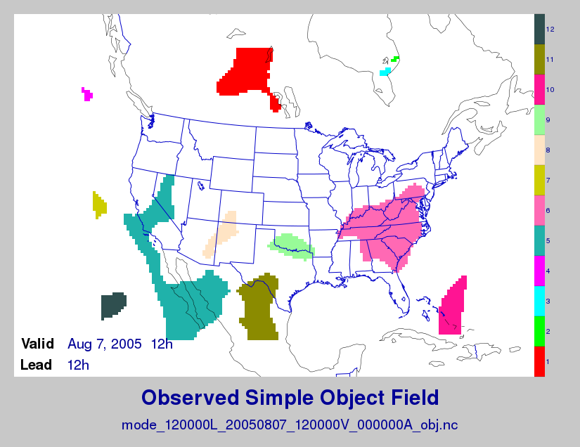
Figure 30.1 Simple observed precipitation objects
Once MET has been applied to forecast and observed fields (or observing locations), and the output has been sorted through the Analysis Tool, numerous graphical and summary analyses can be performed depending on a specific user’s needs. Here we give some examples of graphics and summary scores that one might wish to compute with the given output of MET and MET-TC. Any computing language could be used for this stage; some scripts will be provided on the MET users web page as examples to assist users.
30.2. Examples of plotting MET output
30.2.1. Grid-Stat tool examples
The plots in Figure 30.2 show time series of frequency bias and Gilbert Skill Score, stratified according to time of day. This type of figure is particularly useful for diagnosing problems that are tied to the diurnal cycle. In this case, two of the models (green dash-dotted and black dotted lines) show an especially high Bias (near 3) during the afternoon (15-21 UTC; left panel), while the skill (GSS; right panel) appears to be best for the models represented by the solid black line and green dashed lines in the morning (09-15 UTC). Note that any judgment of skill based on GSS should be restricted to times when the Bias is close to one.
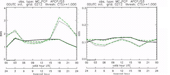
Figure 30.2 Time series of forecast area bias and Gilbert Skill Score for four model configurations (different lines) stratified by time-of-day.
30.2.2. MODE tool examples
When using the MODE tool, it is possible to think of matched objects as hits and unmatched objects as false alarms or misses depending on whether the unmatched object is from the forecast or observed field, respectively. Because the objects can have greatly differing sizes, it is useful to weight the statistics by the areas, which are given in the output as numbers of grid squares. When doing this, it is possible to have different matched observed object areas from matched forecast object areas so that the number of hits will be different depending on which is chosen to be a hit. When comparing multiple forecasts to the same observed field, it is perhaps wise to always use the observed field for the hits so that there is consistency for subsequent comparisons. Defining hits, misses and false alarms in this way allows one to compute many traditional verification scores without the problem of small-scale discrepancies; the matched objects are defined as being matched because they are “close” by the fuzzy logic criteria. Note that scores involving the number of correct negatives may be more difficult to interpret as it is not clear how to define a correct negative in this context. It is also important to evaluate the number and area attributes for these objects in order to provide a more complete picture of how the forecast is performing.
Figure 30.3 gives an example of two traditional verification scores (Bias and CSI) along with bar plots showing the total numbers of objects for the forecast and observed fields, as well as bar plots showing their total areas. These data are from the same set of 13-km WRF model runs analyzed in Figure 30.3. The model runs were initialized at 0 UTC and cover the period 15 July to 15 August 2005. For the forecast evaluation, we compared 3-hour accumulated precipitation for lead times of 3-24 hours to Stage II radar-gauge precipitation. Note that for the 3-hr lead time, indicated as the 0300 UTC valid time in Figure 30.2, the Bias is significantly larger than the other lead times. This is evidenced by the fact that there are both a larger number of forecast objects, and a larger area of forecast objects for this lead time, and only for this lead time. Dashed lines show about 2 bootstrap standard deviations from the estimate.
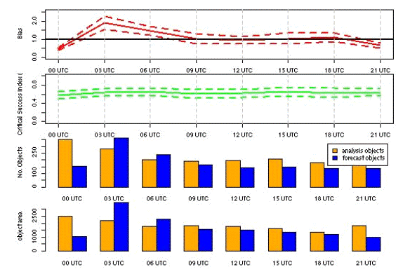
Figure 30.3 Traditional verification scores applied to output of the MODE tool, computed by defining matched observed objects to be hits, unmatched observed objects to be misses, and unmatched forecast objects to be false alarms; weighted by object area. Bar plots show numbers (penultimate row) and areas (bottom row) of observed and forecast objects, respectively.
In addition to the traditional scores, MODE output allows more information to be gleaned about forecast performance. It is even useful when computing the traditional scores to understand how much the forecasts are displaced in terms of both distance and direction. Figure 30.4, for example, shows circle histograms for matched objects. The petals show the percentage of times the forecast object centroids are at a given angle from the observed object centroids. In Figure 30.4 (top diagram) about 25% of the time the forecast object centroids are west of the observed object centroids, whereas in Figure 30.4 (bottom diagram) there is less bias in terms of the forecast objects’ centroid locations compared to those of the observed objects, as evidenced by the petals’ relatively similar lengths, and their relatively even dispersion around the circle. The colors on the petals represent the proportion of centroid distances within each colored bin along each direction. For example, Figure 30.4 (top row) shows that among the forecast object centroids that are located to the West of the observed object centroids, the greatest proportion of the separation distances (between the observed and forecast object centroids) is greater than 20 grid squares.
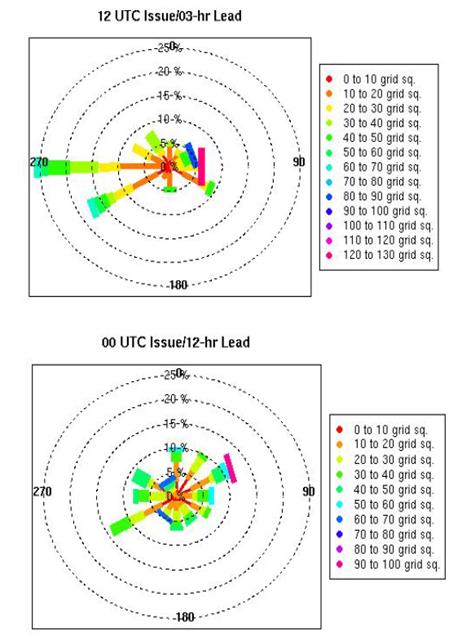
Figure 30.4 Circle histograms showing object centroid angles and distances (see text for explanation).
30.2.3. TC-Stat tool example
There is a basic R script located in the MET installation, share/met/Rscripts/plot_tcmpr.R. The usage statement with a short description of the options for plot_tcmpr.R can be obtained by typing: Rscript plot_tcmpr.R with no additional arguments. The only required argument is the -lookin source, which is the path to the TC-Pairs TCST output files. The R script reads directly from the TC-Pairs output, and calls TC-Stat directly for filter jobs specified in the “-filter options” argument.
In order to run this script, the MET_INSTALL_DIR environment variable must be set to the MET installation directory and the MET_BASE environment variable must be set to the MET_INSTALL_DIR/share/met directory. In addition, the Tc-Stat tool under MET_INSTALL_DIR/bin must be in your system path.
The supplied R script can generate a number of different plot types including boxplots, mean, median, rank, and relative performance. Pairwise differences can be plotted for the boxplots, mean, and median. Normal confidence intervals are applied to all figures unless the no_ci option is set to TRUE. Below are two example plots generated from the tools.
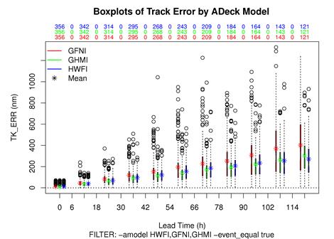
Figure 30.5 Example boxplot from plot_tcmpr.R. Track error distributions by lead time for three operational models GFNI, GHMI, HFWI.
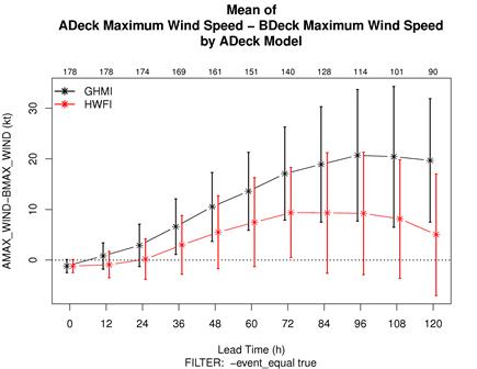
Figure 30.6 Example mean intensity error with confidence intervals at 95% from plot_tcmpr.R. Raw intensity error by lead time for a homogeneous comparison of two operational models GHMI, HWFI.